The Goal
The idea was straightforward: take the raw text of a scientific abstract and automatically decide which broad field it belongs to - computer science, physics, mathematics, biology, and so on. The input data is the public arXiv dataset from Kaggle - roughly 2 million papers, about 4.8 GB of JSONL. The output is a deployed REST API that accepts an abstract and returns a predicted category with a confidence score.
The full stack I landed on:
| Category | Tool |
|---|---|
| Language | Python 3.11 |
| ML Framework | PyTorch + HuggingFace Transformers |
| NLP Preprocessing | NLTK |
| Experiment Tracking | MLflow |
| Hyperparameter Search | Optuna |
| API | Django + Django REST Framework |
| Database | PostgreSQL + pgvector |
| Containerization | Docker + Docker Compose |
| Notebooks | JupyterLab + nbconvert |
Choosing the Model
The obvious starting point for text classification is BERT. But arXiv is entirely scientific literature - filled with domain-specific vocabulary, LaTeX notation, and terminology that a model pre-trained on Wikipedia and BookCorpus has never seen properly.
So instead of bert-base-uncased, I used allenai/scibert_scivocab_uncased - a BERT model pre-trained on ~3.1 million scientific papers from Semantic Scholar. It has the exact same architecture as BERT-base (12 layers, 768 hidden dimensions, 110M parameters), which means inference and fine-tuning costs are identical. The only difference is the vocabulary: SciBERT uses a domain-specific wordpiece vocabulary, so tokens like "eigenvalue", "hep-th", or "convolutional" aren't fragmented into odd subword pieces.
The model head is replaced with a linear classification layer sized to the number of output labels.
Mapping Categories
arXiv uses fine-grained category codes like cs.LG, hep-th, or q-bio.PE. There are hundreds of them. Training a classifier over hundreds of sparse classes on 2M samples would be slow and messy, so I collapsed them into 7 broad domains:
| Domain | arXiv Codes |
|---|---|
| Computer Science | cs.* |
| Physics | hep-*, gr-qc, quant-ph, cond-mat.*, astro-ph.*, nlin.*, nucl-* |
| Mathematics | math.*, stat.* |
| Biology | q-bio.* |
| Economics | econ.*, q-fin.* |
| Engineering | eess.* |
| Other | Everything else |
Only the first (primary) category of each article is used as the label. Most papers have more than one category tag, but the first one consistently reflects the paper's main discipline. This keeps it a clean single-label problem.
The mapping logic uses exact match first (for codes like quant-ph that don't follow the prefix.subcategory pattern), then falls back to a prefix match on the part before the first dot or hyphen. There was one subtle edge case: q-fin.* would match the q prefix and be mapped to Biology if not explicitly handled, since q-bio.* is why q maps there. A few explicit exact-match entries in the lookup table fixed it.
Data Preprocessing
Before the text reaches the HuggingFace tokenizer, it goes through a classic NLP cleaning pipeline implemented in ml/preprocessing.py:
- Unicode NFKC normalisation - arXiv abstracts are LaTeX-heavy; this handles special unicode that otherwise ends up as garbage bytes
- Remove special characters - keeps only letters, digits, and whitespace
- Collapse whitespace - normalises newlines and multiple spaces
- Lowercase
- NLTK word tokenizer
- Remove stop words - English stop words (NLTK corpus)
- Lemmatize - WordNetLemmatizer, reduces inflected forms to base
- Hard truncation - character limit before tokenization
- HuggingFace tokenization - converts to
input_ids+attention_masktensors (max 256 tokens, padded or truncated)
Each step is individually togglable via config flags. All functions are pure with no side effects, so the same pipeline runs identically during training and at inference time.
Training Setup
The dataset is split 80/10/10 (train/val/test) with a fixed seed for reproducibility. Training uses HuggingFace's Trainer API with:
- Optimizer: AdamW
- Scheduler: Linear warmup
- Loss: Cross-entropy
- Evaluation: Every epoch on the validation set
- Early stopping: Stops if validation loss doesn't improve for N consecutive epochs
- Metrics: Accuracy, weighted Precision, weighted Recall, weighted F1
Every training run is logged to MLflow - hyperparameters, per-epoch metrics, and the final model and tokenizer artefacts. The script does a TCP socket probe before trying to connect, so if MLflow is unreachable the run completes normally without any errors.
Saved artefacts:
artifacts/
├── model/                # HuggingFace model weights
├── tokenizer/            # HuggingFace tokenizer
└── metadata/
    ├── label2id.json     # Label ↔ index mapping
    ├── metrics.json      # Final train/val/test metrics
    └── best_hyperparams.json
Hyperparameter Tuning
Hyperparameter search uses HuggingFace Trainer.hyperparameter_search() backed by Optuna. The search space:
learning_rate: log-uniform [1e-5, 5e-5]per_device_train_batch_size: categorical [8, 16, 32]weight_decay: uniform [0.0, 0.3]warmup_ratio: uniform [0.0, 0.2]num_train_epochs: int [2, N]
Each trial is logged to MLflow. Best parameters are saved to artifacts/metadata/best_hyperparams.json.
Challenges Along the Way
Starting with Full Docker
My initial plan was to run everything inside Docker - no Python installation required on the host. This fell apart immediately when it came to training: a Docker container on a laptop has no access to the host GPU. Training on CPU inside Docker on a ~200k sample dataset with a 110M parameter model is impractically slow.
Hybrid Architecture
The solution was a hybrid setup: run the Python-heavy work (training, EDA) natively on the host where it has GPU access, and keep the infrastructure services (PostgreSQL, MLflow, Django) in Docker. Best of both worlds.
Networking After Moving Training Out of Docker
Moving training out of Docker introduced a connectivity issue I hadn't anticipated. Scripts that previously connected to http://mlflow:5000 (Docker's internal DNS) now had to use http://localhost:5001. Two things bit me here:
MLflow v3 binding change: MLflow ≥ 3.1 changed its security middleware to bind to 127.0.0.1 by default, even when --host 0.0.0.0 is passed. The fix was to explicitly pass --workers and --allowed-hosts flags in the MLflow Docker command.
macOS port 5000 conflict: AirPlay Receiver on macOS occupies port 5000. Rather than asking anyone to disable AirPlay, I moved MLflow to port 5001 in docker-compose.yml so the setup works out-of-the-box on Mac.
Apple Silicon GPU Acceleration
Once running natively on an M-series Mac, I added MPS (Metal Performance Shaders) support. The training script auto-detects the device at startup:
if torch.cuda.is_available():
    device_str = "cuda"
    use_fp16, use_bf16 = True, False
elif torch.backends.mps.is_available():
    device_str = "mps"
    use_fp16, use_bf16 = False, True   # M-series supports bf16 natively
else:
    device_str = "cpu"
    use_fp16, use_bf16 = False, False
bf16 (bfloat16) is used instead of fp16 on Apple Silicon because the M-series Neural Engine supports it natively - it halves memory usage and speeds up matrix operations without the numerical instability that fp16 can produce.
One more thing: some PyTorch operations are not yet implemented in Metal. Without setting PYTORCH_ENABLE_MPS_FALLBACK=1, these crash at runtime. With the fallback enabled, unsupported ops transparently execute on CPU for just that step while the rest stays on the GPU.
Results
I ran the full pipeline on two machines to validate cross-platform behaviour.
macOS (M-series, MPS):
Test accuracy:  0.9424
Test F1:        0.9427
Training time:  ~62 minutes (5 epochs)
Samples/sec:    53.5
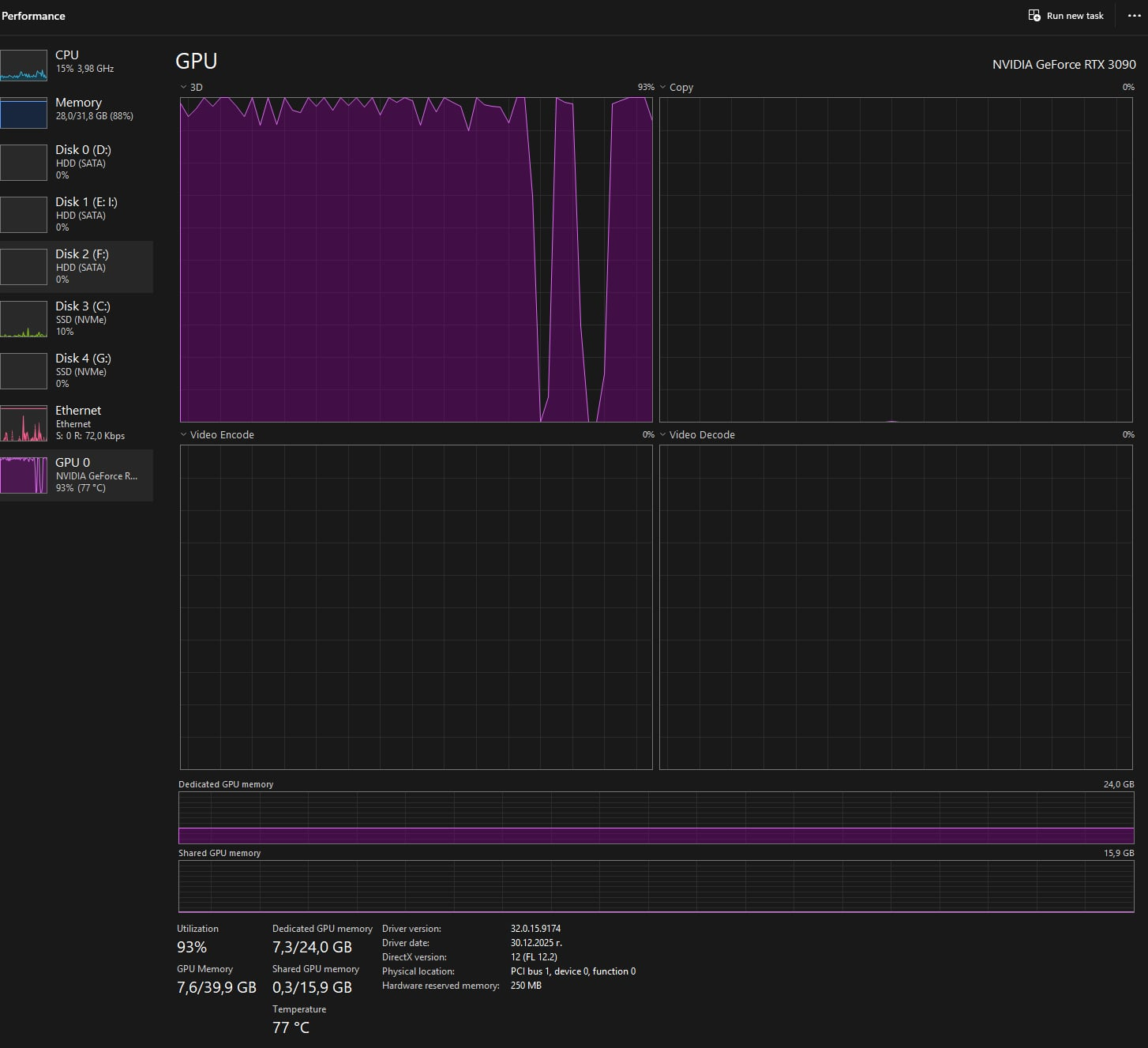
Windows (RTX 3090, CUDA):
Test accuracy:  0.9446
Test F1:        0.9446
Training time:  ~9 minutes (5 epochs)
Samples/sec:    374.3
| Metric | macOS (MPS) | Windows (CUDA) |
|---|---|---|
| Training time (5 epochs) | ~62 min | ~9 min |
| Samples/sec (train) | 53.5 | 374.3 |
| Test accuracy | 0.9424 | 0.9446 |
| Test F1 | 0.9427 | 0.9446 |
The RTX 3090 is roughly 7× faster in training throughput, which matches the difference in train_samples_per_second. More importantly, the model accuracy is essentially identical across both hardware setups - the code path diverges only in device and precision settings, not in the training logic itself.
Both runs reach ~94% test accuracy with balanced precision, recall, and F1 - the model generalises well and isn't simply predicting the majority class.
The REST API
The API is built with Django REST Framework. The model is loaded once on startup via AppConfig.ready() and cached as a singleton - no per-request loading.
Endpoint: POST /api/predict/
Request:
{
  "abstract": "We propose a scalable approach to graph neural networks...",
  "top_k": 3
}
Response:
{
  "predicted_category": "Computer Science",
  "confidence": 0.912,
  "top_k": [
    {"label": "Computer Science", "score": 0.912},
    {"label": "Mathematics", "score": 0.063},
    {"label": "Physics", "score": 0.018}
  ]
}
If the model artefacts aren't present (e.g., training hasn't been run yet), the API returns 503 Service Unavailable with a descriptive message rather than crashing.
A Simple UI
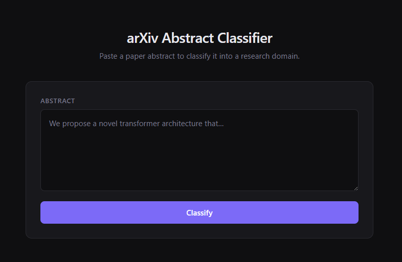
Beyond the API, I added a minimal Django page at / - a dark-themed single-column interface where you can paste an abstract, hit Classify (or Ctrl+Enter / Cmd+Enter), and immediately see the result. It renders the predicted category and confidence prominently, then shows a horizontal bar chart of the top-5 predictions with the winning class highlighted in green. It calls POST /api/predict/ directly from the browser via fetch, so it exercises the same endpoint as any API consumer.
Wrapping Up
The most interesting part of the project wasn't the model - fine-tuning BERT is fairly mechanical once you've done it once. The interesting bits were all in the surrounding infrastructure: dealing with MLflow's changed binding behaviour, the Apple Silicon mixed-precision nuances, the hybrid Docker/native training architecture, and the category mapping edge cases in the arXiv taxonomy.
The final pipeline is fully automated via a single shell script (bash scripts/run_pipeline.sh) that handles dataset download, EDA notebook execution, training, embedding storage, and starting the web server. Flags like --skip-download and --tune let you skip or enable individual steps.
Achieving ~94% accuracy on 7 broad domains with 200k training samples using a model that takes under 10 minutes to train on a mid-range GPU feels like a good result. The consistency across Apple Silicon and CUDA confirms the device-agnostic code path works correctly.
The full source code will be published on GitHub soon - once it's up, you'll be able to clone the repo, point it at the arXiv dataset, and run the entire pipeline end-to-end yourself.